 Time-Domain Processing
 Time-Domain Processing
The simple manipulation of a signal's time-domain representation - it's waveform - can provide a number of useful properties. Some examples of time-domain measurements include energy, average zero-crossing rate and the autocorrelation function (see the auto MAD demonstration). This demonstration will concentrate on the average zero-crossing rate, energy and average magnitude which is closely related to the signal energy (we shall see later that the information they produce is equivalent).
These properties can either used purely as a new way of viewing the information implicitly buried within the signal or as a basis for more complex analysis (for example, in isolated word endpoint detection or pitch estimation). In signal analysis, the act of windowing can have a dramatic influence on the results. The three major aspects are window type, size and shift. This demonstration allows the student to both revise their understanding of the windowing process and also to see how various windowing properties influence the processing techniques.

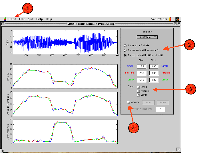
Type 'timedom' to launch the demo. When the window appears, use the load menu (1) to load a sound file. The signal can be played by clicking anywhere within the signal axes. As can be seen, the energy, average magnitude and average zero-crossing rate plots have been created. For each property axes there a 3 different plots - blue, red and green. These correspond to the 3 sets of window properties (2). There are a number of windowing options available:
- 1 window size, with 3 different shifts.
- 3 window sizes, each with the same shift.
- 3 window sizes, each with a different shift. (default)
The individual sizes and shifts together with the window type can be set by the student. Any of the 3 colours can be switched off at any point by using the 'show' checkboxes (3).
The way in which the measurements are made in relation to the windowing of the signal can be investigated by using the animation feature. Click on the 'Animate' checkbox (4). The measurement axes will be cleared and only the appropriate controls will be enabled. Again, the window type, size and shift can be set. To start the animation, click on the 'Run' button. If the animation proceeds too quickly, a pause can be inserted between each segment analysis. A pause of 0 seconds (default) turns off pause-insertion.
Click the 'Animate' checkbox again to revert back to the original interface.
- What do you notice about the energy and average magnitude plots? With reference to their respective defintions, how can your observations be explained?
- What happens to the zero-crossing rate when there is a sharp increase in the energy? What happens when the energy sharply decreases? In the context of speech analysis, what is the reason for this and what types of sounds cause such changes?
- How does the structure of the plots alter when the window sizes and shifts increase? Why?
- Does altering the window type alter the plots? If so, why?
Rabiner, L.R. and Schafer, R.W., "Digital Processing of Speech Signals". Prentice-Hall, 1978, pp. 116-130.
See also the demonstration for autocorrelation (auto).
Produced by: Stuart N Wrigley
Release date: January 20 1999
Permissions: This demonstration may be used and modified freely by anyone. It may be distributed in unmodified form.